How to run simulations with arraylib before arraying a pooled library

The starting point when generating an arrayed library is usually a pooled library which contains a mixture of mutants. Before arraying a pooled library it can be helpful to first run a simulation to estimate how big (how many wells it contains) the arrayed library should be to reach a certain number of mutants with unique genes and second run a simulation to estimate how accurate the deconvolution of the combinatorially pooled arrayed library will be. Both simulations make use of the mutant distribution of the pooled library (i.e. how abundant each mutant is in the starting pooled library). The mutant distribution can be calculated with the tnseeker package and both simulations introduced here expect tnseeker output tables as their input.

import arraylib
import numpy as np

Estimate size of arrayed library to reach a certain number of unique mutants

Run interactively

To run the simulation interactively use the code below.

# perform simulations 10 between 2000 and 5000 mutants
arrsize=np.linspace(2000, 5000,10, dtype=int)

sim_result = arraylib.simulations.simulate_unique_genes(data= "../../tests/test_data/tnseeker_test_output.csv", # path to tnseeker output file
                                            arrsize=arrsize, # arraysizes to simulate (number of mutants/wells in the array)
                                            number_of_repeats=10, # number of repeats for each simulation
                                            gene_start=0.1,
                                            gene_end=0.9, # gene start and end define the range in which a transposon hit is considered to be in a gene
                                            seed=42, # random seed
                                            )

# show output of simulation
sim_result

	Arraysize	Mean	Std
2000	2000	699.8	9.431861
2333	2333	734.9	4.988988
2666	2666	753.6	6.681317
3000	3000	774.2	5.095096
3333	3333	782.5	5.064583
3666	3666	792.7	4.495553
4000	4000	798.9	1.135782
4333	4333	800.6	3.555278
4666	4666	806.1	3.269557
5000	5000	808.2	1.83303

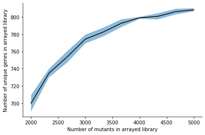
The simulation randomly picks n mutants with probability based on the distribution in the tnseeker output. n is the arrsize, here simulations of array sizes between 2000 and 5000 were performed. Each simulation is repeated number_of_repeats times and the mean and standard deviation of the number of unique genes that were picked among all the picked mutants is calculated. Genes are only counted if the transposon hit it between gene_start and gene_end. We can plot the results:

_ = arraylib.simulations.plot_arraysize_vs_unique_genes(sim_result)

Run on command line

To run the simulation on the command line use:

!arraylib-simulate_required_arraysize ../../tests/test_data/tnseeker_test_output.csv --minsize 2000 --maxsize 5000 --number_of_simulations 10 --number_of_repeats 10 --gene_start 0.1 --gene_end 0.9 --output_filename simulation_output.csv --output_plot simulation_plots.pdf --seed 42

Simulating unique genes for arraysizes between 2000 and 5000 !
Plotting results to simulation_plots.pdf !
Saving results to simulation_output.csv !
Done!

Estimate accuracy of library deconvolution

Run interactively

To run the simulation interactively use the code below. This may take a few minutes.

sim_result = arraylib.simulations.simulate_deconvolution(data= "../../tests/test_data/tnseeker_test_output.csv", # path to tnseeker output file
                                            minsize=2, # minimum gridsize to simulate (gridsize of well plates, e.g. here a grid of wellplates of size 2x2)
                                            maxsize=4, # maximum gridsize
                                            number_of_simulations=2, # number of simulations to run, linearly spaced between minsize and maxsize (here 2 and 4)
                                            seed=42 # random seed
                                            )

# show output of simulation
sim_result

	Arraysize	Precision_4D	Recall_4D	Precision_3D	Recall_3D
384	384	0.869452	0.867188	0.859375	0.859375
1536	1536	0.424384	0.414714	0.476691	0.472656

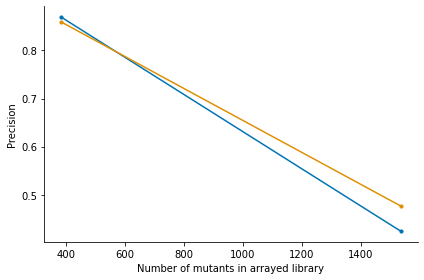
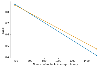
The simulation first arranges a grid 96 well plates. Then for each well of the grid it randomly picks mutants with replacement with probability based on the distribution in the tnseeker output. For each mutant, read counts are simulated and added to the corresponding pools of their given wells. This results in a count matrix with mutants x pools. Then arraylib predicts the locations based on the read counts and calculates precision and recall for the true and predicted locations of the mutants. Precision is the percentage of correctly identified locations among all predicted locations. Recall is the percentage of all the true locations that were predicted. The simulation is performed for a 3D and 4D pooling scheme. We can plot the results using:

_,_ =arraylib.simulations.plot_precision_recall(sim_result)

Run on command line

To run the simulation on the command line use:

!arraylib-simulate_deconvolution ../../tests/test_data/tnseeker_test_output.csv --minsize 2 --maxsize 4 --number_of_simulations 2 --output_filename simulation_output.csv --output_plot simulation_plots.pdf --seed 42

Simulating deconvolution runs for grids of sizes ['2' '4'] !
Plotting results to precision_simulation_plots.pdf !
Plotting results to recall_simulation_plots.pdf !
Saving results to simulation_output.csv !
Done!