![]()
Before you start, make sure to set your runtime type to GPU in colab.
[2]:
# Install SOFA + dependencies
!pip install --quiet biosofa
[1]:
!wget https://zenodo.org/records/14044221/files/pancan_depmap.h5mu?download=1
!mv pancan_depmap.h5mu?download=1 pancan_depmap.h5mu
--2024-11-07 10:03:30--  https://zenodo.org/records/14044221/files/pancan_depmap.h5mu?download=1
Resolving zenodo.org (zenodo.org)... 188.184.98.238, 188.184.103.159, 188.185.79.172, ...
Connecting to zenodo.org (zenodo.org)|188.184.98.238|:443... connected.
HTTP request sent, awaiting response... 200 OK
Length: 79551896 (76M) [application/octet-stream]
Saving to: ‘pancan_depmap.h5mu?download=1’

pancan_depmap.h5mu? 100%[===================>]  75.87M   534KB/s    in 1m 55s

2024-11-07 10:05:26 (677 KB/s) - ‘pancan_depmap.h5mu?download=1’ saved [79551896/79551896]
[29]:
import warnings
warnings.filterwarnings('ignore')
import pandas as pd
import sofa
import numpy as np
import matplotlib.pyplot as plt
import seaborn as sns
import matplotlib
from muon import MuData
import muon as mu
from sklearn.manifold import TSNE
import scanpy as sc
import anndata as ad
from anndata import AnnData
import torch
import seaborn.objects as so
from seaborn import axes_style
Analysis of DepMap data
Introduction
In this notebook we will explore how SOFA can be used to analyze multi-omics data from the DepMap [1,2,3,4,5]. Here we give a brief introduction what the SOFA model does and what it can be used for. For a more detailed description please refer to our preprint: https://doi.org/10.1101/2024.10.10.617527
The SOFA model
Given a set of real-valued data matrices containing multi-omic measurements from overlapping samples (also called views), along with sample-level guiding variables that capture additional properties such as batches or mutational profiles, SOFA extracts an interpretable lower-dimensional data representation, consisting of a shared factor matrix and modality-specific loading matrices. The goal of these factors is to explain the major axes of variation in the data. SOFA explicitly assigns a subset of factors to explain both the multi-omics data and the guiding variables (guided factors), while preserving another subset of factors exclusively for explaining the multi-omics data (unguided factors). Importantly, this feature allows the analyst to discern variation that is driven by known sources from novel, unexplained sources of variability.
Interpretation of the factors (Z)
Analogous to the interpretation of factors in PCA, SOFA factors ordinate samples along a zero-centered axis, where samples with opposing signs exhibit contrasting phenotypes along the inferred axis of variation, and the absolute value of the factor indicates the strength of the phenotype. Importantly, SOFA partitions the factors of the low-rank decomposition into guided and unguided factors: the guided factors are linked to specific guiding variables, while the unguided factors capture global, yet unexplained, sources of variability in the data. The factor values can be used in downstream analysis tasks related to the samples, such as clustering or survival analysis. The factor values are called Z in SOFA.
Interpretation of the loading weights (W)
SOFA’s loading weights indicate the importance of each feature for its respective factor, thereby enabling the interpretation of SOFA factors. Loading weights close to zero indicate that a feature has little to no importance for the respective factor, while large magnitudes suggest strong relevance. The sign of the loading weight aligns with its corresponding factor, meaning that positive loading weights indicate higher feature levels in samples with positive factor values, and negative loading weights indicate higher feature levels in samples with negative factor values. The top loading weights can be simply inspected or used in downstream analysis such as gene set enrichment analysis. The factor values are called W in SOFA.
Supported data
SOFA expects a set of matrices containing omics measurements with matching and aligned samples and different features. Currently SOFA only supports Gaussian likelihoods, for the multi-omics data. Data should therefore be appropriately normalized according to its omics modality. Additionally, data should be centered and scaled.
For the guiding variables SOFA supports Gaussian, Bernoulli and Categorical likelihoods. Guiding variables can therefore be continuous, binary or categorical. Guiding variables should be vectors with matching samples with the multi-omics data.
In SOFA the multi-omics data is denoted as X and the guiding variables as Y.
The DepMap data set
The DepMap project aims to identify cancer vulnerabilities and drug targets across a diverse range of cancer types. The data set includes multi-omics data, encompassing transcriptomics[4], proteomics[1], and methylation[5], as well as drug response profiles for 627 drugs[5] and CRISPR-Cas9 gene essentiality scores[2,3] for 17485 genes for 949 cancer cell lines across 26 different tissues. We will fit a SOFA model with 20 factors, while
accounting for potential/known drivers of variation such as growth rate, microsatellite instability (MSI) status, BRAF, TP53 and PIK3CA mutation and hematopoietic lineage. We will use the essentiality score data test factor associations with essentiality scores. We will first load the preprocessed data in MuData format, fit a SOFA model and perform various downstream analyses.
Read data and set hyperparameters
[2]:
# First we read the preprocessed data as a single MuData object
mdata = mu.read("pancan_depmap.h5mu")
mdata
[2]:
MuData object with n_obs × n_vars = 778 × 23503
  obs:      'DepMap_ID', 'cell_line_name', 'stripped_cell_line_name', 'CCLE_Name', 'alias', 'COSMICID', 'sex', 'source', 'RRID', 'WTSI_Master_Cell_ID', 'sample_collection_site', 'primary_or_metastasis', 'primary_disease', 'Subtype', 'age', 'Sanger_Model_ID', 'depmap_public_comments', 'lineage', 'lineage_subtype', 'lineage_sub_subtype', 'lineage_molecular_subtype', 'default_growth_pattern', 'model_manipulation', 'model_manipulation_details', 'patient_id', 'parent_depmap_id', 'Cellosaurus_NCIt_disease', 'Cellosaurus_NCIt_id', 'Cellosaurus_issues', 'model_id', 'Project_Identifier', 'Cell_line', 'Source', 'Identifier', 'Gender', 'Tissue_type', 'Cancer_type', 'Cancer_subtype', 'Haem_lineage', 'BROAD_ID', 'CCLE_ID', 'ploidy', 'mutational_burden', 'msi_status', 'growth_properties', 'growth', 'size', 'media', 'replicates_correlation', 'number_of_proteins', 'EMT', 'Proteasome', 'TranslationInitiation', 'CopyNumberInstability', 'GeneExpressionCorrelation', 'CopyNumberAttenuation', 'crispr_source', 'hema/lymph'
  12 modalities
    RNA:    778 x 2000
      uns:  'llh', 'log1p'
      obsm: 'mask'
    Protein:        778 x 2000
      uns:  'llh'
      obsm: 'mask'
    Methylation:    778 x 2000
      uns:  'llh', 'log1p'
      obsm: 'mask'
    Drug response:  778 x 627
      uns:  'llh'
      obsm: 'mask'
    CRISPR scores:  778 x 16258
      uns:  'llh'
      obsm: 'mask'
    Mutations:      778 x 612
      uns:  'llh'
      obsm: 'mask'
    Growth: 778 x 1
      uns:  'llh', 'scaling_factor'
      obsm: 'mask'
    MSI:    778 x 1
      uns:  'llh', 'scaling_factor'
      obsm: 'mask'
    BRAF:   778 x 1
      uns:  'llh', 'scaling_factor'
      obsm: 'mask'
    TP53:   778 x 1
      uns:  'llh', 'scaling_factor'
      obsm: 'mask'
    PIK3CA: 778 x 1
      uns:  'llh', 'scaling_factor'
      obsm: 'mask'
    Hema:   778 x 1
      uns:  'llh', 'scaling_factor'
      obsm: 'mask'
The mdata object contains 12 data modalities and the obs slot contains metadata of the cell lines. We will use RNA, Protein, Methylation and Drug response as the multi-omics data input for SOFA. We will use the modalities Growth (the growth rate of the cell lines), MSI (microsatellite instability status), BRAF (whether the cell line is mutated in BRAF), TP53 (whether the cell line is mutated in TP53), PIK3CA (whether the cell line is mutated in PIK3CA) and Hema (whether the cell line is from
the hematopoietic lineage) as guiding variables. The modalities Mutations and CRISPR scores will be used in the downstream analysis, to test for significant associations with factors.
[3]:
# We create the MuData object Xmdata, which contains the multi-omics data:
Xmdata = MuData({"RNA":mdata["RNA"], "Protein":mdata["Protein"], "Methylation":mdata["Methylation"], "Drug response":mdata["Drug response"]})
# We create the MuData objectYmdata, which contains the guiding variables:
Ymdata = MuData({"Growth":mdata["Growth"], "MSI": mdata["MSI"], "BRAF": mdata["BRAF"], "TP53":mdata["TP53"], "PIK3CA":mdata["PIK3CA"], "Hema": mdata["Hema"]})
(Optional for this Tutorial) here we will show how you would prepare the input data for SOFA yourself
We assume that you have a pandas.DataFrame for each of the data modalities.
[4]:
# Extract dataframes from the `MuData` object
rna_df = mdata["RNA"].to_df()
prot_df = mdata["Protein"].to_df()
meth_df = mdata["Methylation"].to_df()
drug_df = mdata["Drug response"].to_df()
Then we can use the sofa.tl.get_ad() function to produce an appropriate AnnData object.
[5]:
rna_ad = sofa.tl.get_ad(rna_df, llh = "gaussian") # currently only the Gaussian likelihood is supported for the omics data
prot_ad = sofa.tl.get_ad(prot_df, llh = "gaussian")
meth_ad = sofa.tl.get_ad(meth_df, llh = "gaussian")
drug_ad = sofa.tl.get_ad(drug_df, llh = "gaussian")
# Finally as before wrap all the `AnnData` objects in a single `MuData` object.
Xmdata = MuData({"RNA":rna_ad, "Protein":prot_ad, "Methylation":meth_ad, "Drug response":drug_ad})
and analogously for the guiding variables:
[6]:
growth_df = mdata["Growth"].to_df()
msi_df = mdata["MSI"].to_df()
braf_df = mdata["BRAF"].to_df()
tp53_df = mdata["TP53"].to_df()
pik3ca_df = mdata["PIK3CA"].to_df()
hema_df = mdata["Hema"].to_df()
Again we can use the sofa.tl.get_ad() function to produce an appropriate AnnData object. We need to specify an appropriate likelihood for each guiding variables. For the continuous growth rate we use gaussian and for the remaining binary variables bernoulli. SOFA also supports the categorical likelihood. Additionally, we need to set a scaling factor for each guiding variables, determining the strength of the supervision in the fitting process. To high values lead to guided
factors that do not explain any variance of the multi-omics data. Too low values would lead to factors that are not associated with their guiding variables. We recommend the default of 0.1.
[7]:
growth_ad = sofa.tl.get_ad(growth_df, llh = "gaussian", scaling_factor = 0.01)
msi_ad = sofa.tl.get_ad(msi_df, llh = "bernoulli", scaling_factor = 0.1)
braf_ad = sofa.tl.get_ad(braf_df, llh = "bernoulli", scaling_factor = 0.1)
tp53_ad = sofa.tl.get_ad(tp53_df, llh = "bernoulli", scaling_factor = 0.1)
pik3ca_ad = sofa.tl.get_ad(pik3ca_df, llh = "bernoulli", scaling_factor = 0.1)
hema_ad = sofa.tl.get_ad(hema_df, llh = "bernoulli", scaling_factor = 0.1)

# Finally as before wrap all the `AnnData` objects in a single `MuData` object.
Ymdata = MuData({"Growth":growth_ad, "MSI": msi_ad, "BRAF": braf_ad, "TP53": tp53_ad, "PIK3CA": pik3ca_ad, "Hema": hema_ad})
[40]:
# We set the number of factors to infer
num_factors = 20
# Use obs as metadata of the cell lines
metadata = mdata.obs
# In order to relate factors to guiding variables we need to provide a design matrix (guiding variables x number of factors)
# indicating which factor is guided by which guiding variable.
# Here we just indicate that the first 6 factors are each guided by a different guiding variable:
design = np.zeros((len(Ymdata.mod), num_factors))
for i in range(len(Ymdata.mod)):
    design[i,i] = 1

# convert to torch tensor to make it usable by SOFA
design = torch.tensor(design)
design
[40]:
tensor([[1., 0., 0., 0., 0., 0., 0., 0., 0., 0., 0., 0., 0., 0., 0., 0., 0., 0.,
         0., 0.],
        [0., 1., 0., 0., 0., 0., 0., 0., 0., 0., 0., 0., 0., 0., 0., 0., 0., 0.,
         0., 0.],
        [0., 0., 1., 0., 0., 0., 0., 0., 0., 0., 0., 0., 0., 0., 0., 0., 0., 0.,
         0., 0.],
        [0., 0., 0., 1., 0., 0., 0., 0., 0., 0., 0., 0., 0., 0., 0., 0., 0., 0.,
         0., 0.],
        [0., 0., 0., 0., 1., 0., 0., 0., 0., 0., 0., 0., 0., 0., 0., 0., 0., 0.,
         0., 0.],
        [0., 0., 0., 0., 0., 1., 0., 0., 0., 0., 0., 0., 0., 0., 0., 0., 0., 0.,
         0., 0.]], dtype=torch.float64)
Fit the SOFA model
[9]:
model = sofa.SOFA(Xmdata = Xmdata, # the input multi-omics data
                  num_factors=num_factors, # number of factors to infer
                  Ymdata = Ymdata, # the input guiding variables
                  design = design, # design matrix relating factors to guiding variables
                  device='cuda', # set device to "cuda" to enable computation on the GPU, if you don't have a GPU available set it to "cpu"
                  seed=42) # set seed to get the same results every time we run it
[ ]:
# train SOFA with learning rate of 0.01 for 3000 steps
model.fit(n_steps=3000, lr=0.01)
# decrease learning rate to 0.005 and continue training
model.fit(n_steps=3000, lr=0.005)
[12]:
# if we would like to save the fitted model we can save it using:
#sofa.tl.save_model(model,"depmap_example_model")

# to load the model use:
model = sofa.tl.load_model("depmap_example_model")
Downstream analysis
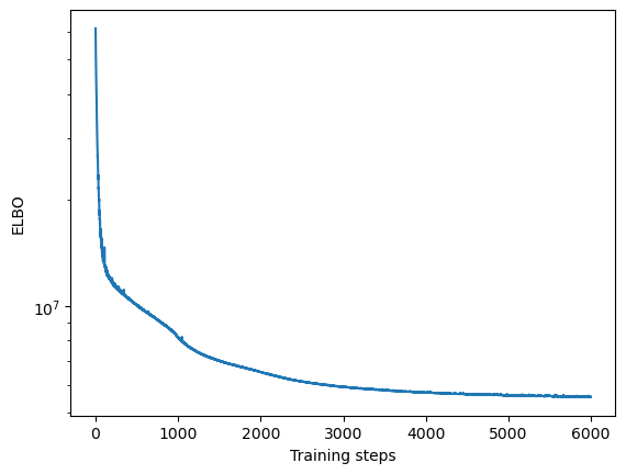
Convergence
We will first assess whether the ELBO loss of SOFA has converged by plotting it over training steps
[13]:
plt.semilogy(model.history)
plt.xlabel("Training steps")
plt.ylabel("ELBO")
[13]:
Text(0, 0.5, 'ELBO')
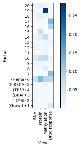
Variance explained
A good first step in a SOFA analysis is to plot how much variance is explained by each factor for each modality. This gives us an overview which factors are active across multiple modalities, capturing correlated variation across multiple measurements and which are private to a single modality, most probably capturing technical effects related to this modality.
[16]:
sofa.pl.plot_variance_explained(model)
[16]:
<Axes: xlabel='View', ylabel='Factor'>
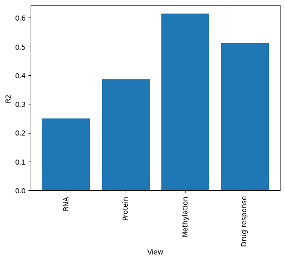
[13]:
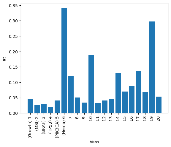
# We can also plot how much variance of each view is explained
sofa.pl.plot_variance_explained_view(model)
[13]:
<Axes: xlabel='View', ylabel='R2'>
[14]:
# or how much variance is explained by each factor in total
sofa.pl.plot_variance_explained_factor(model)
[14]:
<Axes: xlabel='View', ylabel='R2'>
Check factor guidance
[23]:
# concatenate metadata with TP53, BRAF and PIK3CA mutation columns
metadata= pd.concat((metadata, mdata.mod["Mutations"].to_df()[["TP53", "BRAF", "PIK3CA"]]), axis=1)
[24]:
# plot correlation of factor values with selected metadata variables ["growth", "msi_status","BRAF","TP53",  "PIK3CA", "hema/lymph"]
sofa.pl.plot_factor_metadata_cor(model, metadata[["growth", "msi_status","BRAF","TP53",  "PIK3CA", "hema/lymph"]])
[24]:
<Axes: xlabel='Covariate', ylabel='Factor'>
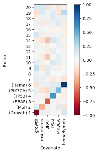
As expected the guided factors a correlated with their respective guiding variables. The unguided factors are not correlated with the guiding variables. Additionally we can check whether guided factors separate by their guiding variables:
[41]:
metadata= pd.concat((metadata, mdata.mod["Mutations"].to_df()[["TP53", "BRAF", "PIK3CA"]]), axis=1)
indicator = pd.concat([
    metadata.loc[:, ['msi_status']].assign(binary=lambda df: df['msi_status'].map({'MSS': 0, 'MSI': 1}).astype(float)).assign(Factor=2).drop(columns='msi_status'),
    metadata.loc[:, ['BRAF']].rename(columns={'BRAF': 'binary'}).assign(binary=lambda df: df['binary'].astype(float)).assign(Factor=3),
    metadata.loc[:, ['TP53']].rename(columns={'TP53': 'binary'}).assign(binary=lambda df: df['binary'].astype(float)).assign(Factor=4),
    metadata.loc[:, ['PIK3CA']].rename(columns={'PIK3CA': 'binary'}).assign(binary=lambda df: df['binary'].astype(float)).assign(Factor=5),
    metadata.loc[:, ['hema/lymph']].assign(binary=lambda df: df['hema/lymph'].map({'other': 0, 'hematopoeitic': 1})).assign(binary=lambda df: df['binary'].astype(float)).assign(Factor=6).drop(columns='hema/lymph')
]
).reset_index()

factor_df = pd.DataFrame(model.Z, index=metadata.index, columns=[i for i in range(1, 21)])

guided_factor_df = (factor_df
 .reset_index()
 .melt('index', var_name='Factor', value_name='Value')
 .merge(indicator, on=['index', 'Factor'])
)
[45]:
fig, ax = plt.subplots()
p1 = (
    so.Plot(guided_factor_df, x='Factor', y='Value', color='binary')
    .add(so.Dot(pointsize=5),  so.Jitter(.3), legend=True)
    .scale(color=so.Nominal())
    .theme(axes_style("white"))
)

p1.on(ax).plot() #.show()


ax.set_title('Guided factors')
ax.set_xticks(range(2,7))
ax.set_ylabel("Factor value")
ax.set_ylim(top=4)
ax.spines['top'].set_visible(False)
ax.spines['right'].set_visible(False)
plt.tight_layout()
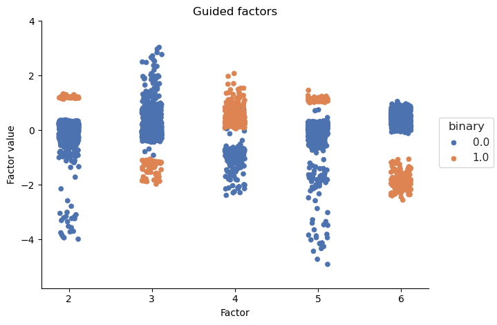
Guided Factors clearly separate by their binary guiding variables, indicating that factor guidance worked.
Downstream analysis of the factor values
The factor values represent the new coordinates in lower dimensional space of our samples and have dimensions samples x factors. The factor values called Z in SOFA. We can use the factor values for all kinds of downstream analyses on the sample level. Here we will cluster the unguided factors.
We first retrieve the factor values:
[17]:
Z = sofa.tl.get_factors(model)
Z
[17]:
| Factor_0 (Growth) | Factor_1 (MSI) | Factor_2 (BRAF) | Factor_3 (TP53) | Factor_4 (PIK3CA) | Factor_5 (Hema) | Factor_6 | Factor_7 | Factor_8 | Factor_9 | Factor_10 | Factor_11 | Factor_12 | Factor_13 | Factor_14 | Factor_15 | Factor_16 | Factor_17 | Factor_18 | Factor_19 | |
|---|---|---|---|---|---|---|---|---|---|---|---|---|---|---|---|---|---|---|---|---|
| 0 | -0.984563 | 0.094903 | 1.867936 | 0.991292 | -0.005510 | 0.174301 | -0.149569 | -0.101285 | 0.118306 | 0.228873 | -0.208032 | -0.263638 | -0.600392 | -0.382208 | 0.140103 | 0.344184 | -0.815846 | 0.459298 | 0.719330 | -0.313031 |
| 1 | -0.674658 | 0.031586 | -0.789824 | -0.407347 | 1.124087 | 0.458733 | -0.060520 | -0.040364 | -0.503078 | -0.399277 | 0.166812 | -0.032913 | 0.652486 | -0.614164 | 0.154161 | 0.377786 | 0.100994 | -1.004648 | -0.408009 | 0.504229 |
| 2 | -0.361459 | -0.191929 | -0.307024 | 0.383602 | 0.018404 | 0.897071 | 0.294184 | -0.372404 | 0.148475 | 0.785472 | -0.204483 | 0.098536 | 0.097677 | 0.411425 | -0.391176 | 0.374827 | 0.386192 | -0.456484 | 0.346030 | 0.550844 |
| 3 | -0.605062 | -0.200432 | -0.299046 | 0.202695 | 0.221496 | 0.108696 | -0.091975 | 0.026284 | 0.158653 | 0.096715 | 0.113269 | -0.056898 | -0.152790 | 0.209436 | 0.354010 | 0.336211 | 0.376640 | -0.477210 | -0.379058 | 0.468571 |
| 4 | 0.212342 | -0.120816 | -0.212216 | 0.690939 | 0.186770 | 0.897576 | 0.123370 | 0.123256 | -0.111156 | 0.608043 | -0.065553 | 0.236904 | -0.198532 | -0.240049 | -0.649414 | 0.371791 | 0.641309 | 0.105965 | 0.207381 | 0.464103 |
| ... | ... | ... | ... | ... | ... | ... | ... | ... | ... | ... | ... | ... | ... | ... | ... | ... | ... | ... | ... | ... |
| 773 | -0.030411 | -0.103553 | -0.316009 | 0.223481 | 0.244809 | 0.518574 | 0.131121 | -0.026001 | -0.492095 | -0.288541 | 0.167538 | 0.161157 | 0.659408 | -0.443171 | 0.323169 | -0.498860 | -0.499177 | -1.300491 | 0.662859 | 0.273217 |
| 774 | 0.561793 | -0.662839 | 0.209959 | -0.977655 | 0.237925 | 0.574140 | -0.069846 | 0.001591 | -1.813954 | 0.000474 | -0.044735 | 0.296505 | -0.099778 | 0.061658 | 0.567360 | 0.424479 | -0.512040 | 1.120325 | -0.449671 | -1.028471 |
| 775 | 0.208128 | -0.140388 | 0.508802 | -0.937757 | -0.153248 | -2.141505 | -0.047474 | 0.235640 | 0.024192 | -0.118403 | -0.061317 | -0.530468 | 0.032437 | -0.095084 | -0.306878 | -0.375194 | 0.274054 | 0.427416 | -1.491817 | 0.362090 |
| 776 | 1.427114 | -1.299472 | -0.234395 | -0.894223 | 0.246734 | 0.601628 | 0.543358 | 0.153857 | -1.782104 | 0.350788 | 0.240557 | 0.425656 | -0.485319 | 0.379114 | -0.334070 | -0.889224 | 0.031068 | 0.376890 | -0.444826 | -0.905731 |
| 777 | -0.233796 | 0.198935 | 2.749278 | 1.159026 | -0.625919 | 0.637330 | -0.659517 | 1.177139 | 0.177545 | 0.033086 | -0.106065 | -0.191898 | -0.288880 | -1.048721 | -0.279230 | 0.333567 | 0.657307 | 0.193587 | 2.300986 | -0.597988 |
778 rows × 20 columns
We will plot a tSNE of all the factors and color them by cancer type:
[18]:
tsne = TSNE()
tsne_z = tsne.fit_transform(model.Z)
[19]:
fig,ax = plt.subplots(1)

for i in np.unique(metadata["lineage"].astype(str)):
    ax.scatter(tsne_z[metadata["lineage"].astype(str)==i,0],tsne_z[metadata["lineage"].astype(str)==i,1], s =10, alpha=0.8,label=i)
ax.set_aspect("equal")
ax.set_xlabel("tSNE 1")
ax.set_ylabel("tSNE 2")
ax.tick_params(
    axis='both',          # changes apply to the x-axis
    which='both',      # both major and minor ticks are affected
    bottom=False,      # ticks along the bottom edge are off
    top=False,
    left=False,# ticks along the top edge are off
    labelbottom=False,
labelleft=False,)
ax.spines[['top','right','left','bottom']].set_visible(False)
ax.legend(frameon=False, ncols=2, loc="center left",bbox_to_anchor=(1,0.5))
[19]:
<matplotlib.legend.Legend at 0x7ff8445060d0>

Downstream analysis of loading weights
The loadings capture the importance of the features in each omics modality for each factor, they have dimensions: factors x features. To retrieve the loadings run:
[9]:
# specify the view of which we want to retrieve the loadings
W = sofa.tl.get_loadings(model, view="RNA")
W
[9]:
| symbol | A2M | AADACL2 | AADACL3 | AARD | ABCB10P1 | ABI3BP | ACAN | ACKR3 | ACP3 | ACTA2 | ... | XBP1 | XCL2 | ZNF683 | ZNF723 | ZNRF4 | ZP2 | ZP4 | ZPLD1 | ZSCAN10 | ZSWIM5P3 |
|---|---|---|---|---|---|---|---|---|---|---|---|---|---|---|---|---|---|---|---|---|---|
| 0 | 0.015295 | 0.071497 | 0.035568 | 0.089748 | -0.044069 | 0.073249 | 0.057849 | 0.014150 | -0.007009 | -0.008777 | ... | -0.029756 | 0.015113 | 0.042406 | 0.026360 | 0.010476 | -0.007051 | -0.005228 | -0.024504 | 0.009037 | 0.015518 |
| 1 | -0.034314 | -0.000051 | 0.023871 | -0.097714 | 0.070291 | -0.047070 | 0.091474 | -0.057706 | -0.268044 | -0.026221 | ... | -0.037763 | 0.029878 | 0.045231 | -0.062290 | -0.131012 | -0.080212 | -0.024728 | -0.048543 | 0.021252 | -0.004852 |
| 2 | -0.321572 | 0.045532 | 0.004737 | -0.070684 | -0.024462 | -0.011495 | -0.150803 | 0.258310 | -0.023645 | 0.054582 | ... | 0.071099 | 0.111338 | 0.020180 | -0.049511 | -0.059965 | 0.063550 | -0.019318 | 0.126384 | 0.001582 | 0.015054 |
| 3 | -0.009988 | -0.003648 | 0.012213 | 0.121117 | 0.031789 | -0.031690 | -0.033959 | 0.002975 | -0.057448 | -0.136400 | ... | -0.068956 | 0.031779 | 0.245507 | 0.027935 | 0.038758 | -0.057646 | -0.054516 | -0.055807 | -0.005945 | -0.003330 |
| 4 | -0.104526 | 0.066071 | 0.052031 | 0.007025 | 0.083235 | 0.038949 | -0.075813 | 0.105265 | 0.076275 | 0.093963 | ... | -0.027402 | 0.041936 | 0.013638 | 0.020756 | 0.009367 | 0.003728 | 0.026330 | 0.006912 | 0.076745 | -0.143186 |
| 5 | 0.102369 | 0.060284 | 0.038335 | 0.013700 | -0.111408 | 0.278752 | 0.066290 | 0.134587 | -0.168386 | 0.098990 | ... | -0.064056 | -0.045495 | -0.201629 | -0.056866 | -0.007317 | -0.084082 | -0.051703 | 0.098773 | -0.122135 | -0.010227 |
| 6 | -0.177834 | -0.042088 | 0.000444 | 0.010341 | 0.108204 | 0.005978 | 0.027057 | -0.006823 | -0.105048 | -0.166809 | ... | 0.147754 | -0.021945 | 0.199206 | 0.040381 | -0.033136 | -0.052512 | 0.018241 | -0.003154 | 0.250065 | -0.082886 |
| 7 | 0.064315 | -0.179968 | 0.041989 | -0.258878 | -0.158774 | 0.052421 | 0.052402 | -0.184161 | -0.064313 | -0.016940 | ... | 0.120286 | -0.008686 | -0.231400 | 0.272920 | -0.021050 | 0.109255 | 0.118702 | 0.021676 | -0.181603 | -0.013686 |
| 8 | 0.022922 | 0.312208 | 0.010867 | -0.191499 | 0.106837 | -0.229320 | -0.008715 | -0.210733 | 0.037657 | 0.062167 | ... | 0.085694 | 0.040236 | -0.080379 | -0.042302 | 0.103474 | -0.319116 | 0.086957 | -0.002122 | 0.176039 | -0.005275 |
| 9 | -0.307194 | 0.043982 | 0.100535 | -0.267381 | -0.050292 | -0.010615 | -0.169009 | 0.112214 | 0.375080 | -0.178900 | ... | 0.012742 | -0.063244 | -0.010274 | -0.093946 | -0.064835 | 0.015574 | 0.066980 | 0.022103 | -0.124436 | -0.030850 |
| 10 | -0.460474 | -0.161775 | 0.248694 | 0.026441 | 0.160128 | 0.045803 | -0.233451 | -0.090797 | 0.112407 | 0.233218 | ... | 0.098966 | -0.276042 | -0.014679 | 0.299511 | 0.042258 | -0.020505 | -0.006881 | -0.029953 | 0.251095 | 0.169541 |
| 11 | -0.011533 | 0.112840 | 0.052935 | -0.015447 | -0.496742 | -0.003645 | 0.026647 | 0.325467 | -0.001202 | 0.038805 | ... | 0.125546 | -0.109403 | -0.441826 | -0.083174 | -0.185597 | -0.014198 | 0.024846 | -0.064795 | 0.087614 | 0.030194 |
| 12 | 0.245613 | 0.296580 | -0.038640 | -0.305640 | -0.124200 | 0.271039 | 0.256376 | 0.541047 | 0.342560 | 0.444382 | ... | 0.560416 | -0.040864 | -0.018886 | -0.035057 | 0.008567 | 0.115618 | 0.088392 | -0.240834 | -0.047551 | -0.004341 |
| 13 | -0.660592 | 0.019101 | -0.120316 | -0.134759 | -0.079046 | -0.341223 | -0.456594 | -0.103917 | 0.044514 | -0.499875 | ... | 0.023534 | 0.128351 | -0.001446 | -0.276361 | 0.020640 | 0.088788 | -0.147279 | -0.029944 | 0.029581 | 0.008861 |
| 14 | -0.085970 | -0.005224 | -0.109311 | -0.124855 | 0.053398 | 0.029236 | -0.034264 | -0.209597 | 0.003543 | -0.030162 | ... | 0.104430 | -0.231496 | -0.059287 | -0.001135 | 0.046376 | 0.015712 | -0.034782 | -0.005570 | 0.020778 | -0.011761 |
| 15 | -0.010765 | -0.039279 | -0.028720 | 0.005197 | -0.021794 | -0.020378 | 0.005175 | 0.006982 | 0.017629 | -0.019821 | ... | -0.011246 | 0.008254 | 0.046750 | 0.060618 | 0.022018 | -0.094701 | 0.021379 | -0.037993 | -0.040373 | -0.096038 |
| 16 | -0.102186 | 0.118045 | 0.007831 | 0.033710 | 0.026295 | -0.103503 | -0.186066 | -0.038786 | 0.027735 | -0.093989 | ... | -0.233836 | 0.137448 | 0.046462 | -0.017949 | -0.011706 | -0.010605 | 0.010610 | -0.056985 | 0.004476 | 0.000662 |
| 17 | -0.133406 | 0.200971 | 0.115494 | 0.210792 | 0.246593 | -0.616548 | -0.265424 | 0.108277 | 0.383489 | -0.634510 | ... | 0.005781 | 0.341722 | -0.029150 | 0.164946 | -0.003980 | 0.146180 | 0.165554 | -0.024582 | -0.000005 | -0.012273 |
| 18 | -0.031818 | 0.005847 | 0.032746 | -0.134567 | 0.327935 | 0.030983 | -0.019491 | 0.083426 | 0.073085 | -0.001174 | ... | -0.062192 | 0.260967 | -0.008846 | 0.142483 | -0.016763 | -0.008566 | -0.008396 | -0.053864 | 0.054478 | 0.011180 |
| 19 | -0.600847 | 0.053716 | 0.075986 | -0.049103 | 0.048417 | 0.555588 | -0.332565 | 0.418213 | -0.372007 | 0.248540 | ... | -0.052842 | 0.318683 | -0.009427 | 0.426128 | -0.065958 | -0.097275 | 0.261584 | 0.066420 | -0.060836 | 0.083081 |
20 rows × 2000 columns
[ ]:
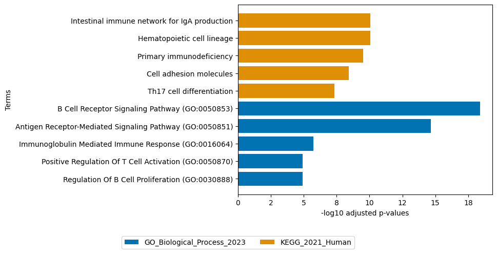
# to get the names of the top 100 negative loadings of factor 5 (guided by hematopoietic lineage) of the RNA modality run:
top_loadings = sofa.tl.get_top_loadings(model, view="RNA", factor = 6, top_n=100, sign="-")
# this can be useful to perform gene overrepresentation analysis:
sofa.pl.plot_enrichment(top_loadings, # the top features
                        background=mdata.mod["RNA"].var, # all genes considered in the analysis, used as background
                        db=["GO_Biological_Process_2023", "KEGG_2021_Human"], # a list of databases for overrepresentation analysis,
                        top_n=[5,5]) # the number of genesets for each database to plot
# sofa.pl.plot_enrichment uses the enrichr API, please refer to https://maayanlab.cloud/Enrichr/#libraries for a full list of available databases
<Axes: xlabel='-log10 adjusted p-values', ylabel='Terms'>
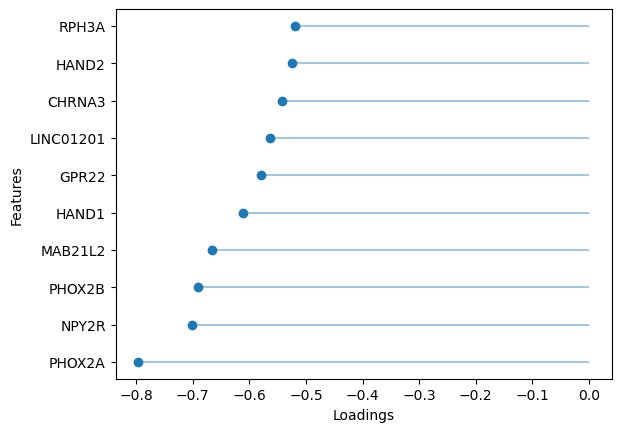
[ ]:
sofa.pl.plot_top_loadings(model, view="RNA", factor = 5, top_n=10, sign="-")
<Axes: xlabel='Loadings', ylabel='Features'>
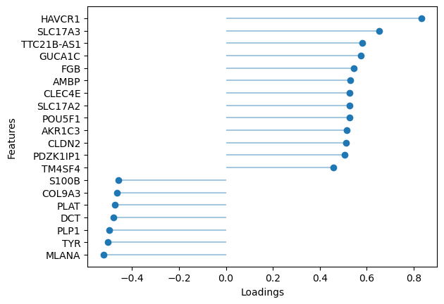
If we omit the sign, the top absolute loading values are shown, in this case both positive and negative for Factor 3 (BRAF mutation)
[55]:
sofa.pl.plot_top_loadings(model, view="RNA", factor = 3, top_n=20)
[55]:
<Axes: xlabel='Loadings', ylabel='Features'>