![]()
Before you start, make sure to set your runtime type to GPU in colab.
[25]:
# Install SOFA + dependencies
!pip install --quiet biosofa
[1]:
# download data
!wget https://datasets.cellxgene.cziscience.com/484dbc33-c7dc-4e5e-9954-7f2a1cc849bc.h5ad # RNA-Seq
!mv 484dbc33-c7dc-4e5e-9954-7f2a1cc849bc.h5ad rna.h5ad
!wget https://datasets.cellxgene.cziscience.com/fecbd715-66f5-48ae-8c39-51a76d7f1d3d.h5ad # ATAC-Seq
!mv fecbd715-66f5-48ae-8c39-51a76d7f1d3d.h5ad atac.h5ad
--2024-11-06 09:37:23--  https://datasets.cellxgene.cziscience.com/484dbc33-c7dc-4e5e-9954-7f2a1cc849bc.h5ad
Resolving datasets.cellxgene.cziscience.com (datasets.cellxgene.cziscience.com)... 18.172.112.45, 18.172.112.61, 18.172.112.87, ...
Connecting to datasets.cellxgene.cziscience.com (datasets.cellxgene.cziscience.com)|18.172.112.45|:443... connected.
HTTP request sent, awaiting response... 200 OK
Length: 405964465 (387M) [binary/octet-stream]
Saving to: ‘484dbc33-c7dc-4e5e-9954-7f2a1cc849bc.h5ad’

-c7dc-4e5e-9954-7f2  24%[===>                ]  95.62M  22.3MB/s    eta 17s    ^C
--2024-11-06 09:37:30--  https://datasets.cellxgene.cziscience.com/fecbd715-66f5-48ae-8c39-51a76d7f1d3d.h5ad
Resolving datasets.cellxgene.cziscience.com (datasets.cellxgene.cziscience.com)... 18.172.112.45, 18.172.112.61, 18.172.112.87, ...
Connecting to datasets.cellxgene.cziscience.com (datasets.cellxgene.cziscience.com)|18.172.112.45|:443... connected.
HTTP request sent, awaiting response... 200 OK
Length: 906950703 (865M) [binary/octet-stream]
Saving to: ‘fecbd715-66f5-48ae-8c39-51a76d7f1d3d.h5ad’

    fecbd715-66f5-4   2%[                    ]  20.59M  12.2MB/s               ^C
[1]:
import warnings
warnings.filterwarnings('ignore')

import sofa
import torch
import pandas as pd
import numpy as np
import matplotlib.pyplot as plt
import seaborn as sns
import matplotlib
from sklearn.preprocessing import StandardScaler, OneHotEncoder
from muon import MuData
from sklearn.manifold import TSNE
import matplotlib.patches as mpatches
import scanpy as sc
import anndata as ad
from anndata import AnnData
import muon
from matplotlib import colors as mp_colors
Analysis of a single-cell multiome data set
Introduction
In this notebook we will explore how SOFA can be used to analyze multi-omics data from the DepMap [1,2,3,4,5]. Here we give a brief introduction what the SOFA model does and what it can be used for. For a more detailed description please refer to our preprint: https://doi.org/10.1101/2024.10.10.617527
The SOFA model
Given a set of real-valued data matrices containing multi-omic measurements from overlapping samples (also called views), along with sample-level guiding variables that capture additional properties such as batches or mutational profiles, SOFA extracts an interpretable lower-dimensional data representation, consisting of a shared factor matrix and modality-specific loading matrices. The goal of these factors is to explain the major axes of variation in the data. SOFA explicitly assigns a subset of factors to explain both the multi-omics data and the guiding variables (guided factors), while preserving another subset of factors exclusively for explaining the multi-omics data (unguided factors). Importantly, this feature allows the analyst to discern variation that is driven by known sources from novel, unexplained sources of variability.
Interpretation of the factors (Z)
Analogous to the interpretation of factors in PCA, SOFA factors ordinate samples along a zero-centered axis, where samples with opposing signs exhibit contrasting phenotypes along the inferred axis of variation, and the absolute value of the factor indicates the strength of the phenotype. Importantly, SOFA partitions the factors of the low-rank decomposition into guided and unguided factors: the guided factors are linked to specific guiding variables, while the unguided factors capture global, yet unexplained, sources of variability in the data. The factor values can be used in downstream analysis tasks related to the samples, such as clustering or survival analysis. The factor values are called Z in SOFA.
Interpretation of the loading weights (W)
SOFA’s loading weights indicate the importance of each feature for its respective factor, thereby enabling the interpretation of SOFA factors. Loading weights close to zero indicate that a feature has little to no importance for the respective factor, while large magnitudes suggest strong relevance. The sign of the loading weight aligns with its corresponding factor, meaning that positive loading weights indicate higher feature levels in samples with positive factor values, and negative loading weights indicate higher feature levels in samples with negative factor values. The top loading weights can be simply inspected or used in downstream analysis such as gene set enrichment analysis. The factor values are called W in SOFA.
Supported data
SOFA expects a set of matrices containing omics measurements with matching and aligned samples and different features. Currently SOFA only supports Gaussian likelihoods, for the multi-omics data. Data should therefore be appropriately normalized according to its omics modality. Additionally, data should be centered and scaled.
For the guiding variables SOFA supports Gaussian, Bernoulli and Categorical likelihoods. Guiding variables can therefore be continuous, binary or categorical. Guiding variables should be vectors with matching samples with the multi-omics data.
In SOFA the multi-omics data is denoted as X and the guiding variables as Y.
Single-cell multiome data set of the human cortex
The data we analyze in this notebook was generated by [1]. The authors simultaneously profiled the transcriptome (RNA) and chromatin accessibility (ATAC) of 45549 single cells of the human cerebral cortex at 6 different developmental stages. The authors identified 13 different cell types in the data. We will fit a SOFA model with 15 factors and guide the first 13 factors with a different cell type label. The 13 guided factors will explain the molecular differences between the cell types, while the 2 unguided factors are free to explain within cell type variation. We will first load the data and do some basic preprocessing, then fit a SOFA model and perform various downstream analyses.
[1] Zhu, K. et al. Multi-omic profiling of the developing human cerebral cortex at the single-cell level. Sci Adv 9, eadg3754 (2023).
Load and preprocess
[4]:
adata_rna= sc.read_h5ad("rna.h5ad")
[5]:
adata_rna
[5]:
AnnData object with n_obs × n_vars = 45549 × 30113
    obs: 'author_cell_type', 'age_group', 'donor_id', 'nCount_RNA', 'nFeature_RNA', 'nCount_ATAC', 'nFeature_ATAC', 'TSS_percentile', 'nucleosome_signal', 'percent_mt', 'assay_ontology_term_id', 'cell_type_ontology_term_id', 'development_stage_ontology_term_id', 'disease_ontology_term_id', 'self_reported_ethnicity_ontology_term_id', 'organism_ontology_term_id', 'sex_ontology_term_id', 'tissue_ontology_term_id', 'suspension_type', 'is_primary_data', 'batch', 'tissue_type', 'cell_type', 'assay', 'disease', 'organism', 'sex', 'tissue', 'self_reported_ethnicity', 'development_stage', 'observation_joinid'
    var: 'feature_is_filtered', 'feature_name', 'feature_reference', 'feature_biotype', 'feature_length'
    uns: 'batch_condition', 'citation', 'schema_reference', 'schema_version', 'title'
    obsm: 'X_joint_wnn_umap', 'X_umap'
[6]:
# basic preprocessing
adata_rna.X = adata_rna.raw.X
# normalization to total library size
sc.pp.normalize_total(adata_rna)
# log transformation
sc.pp.log1p(adata_rna)
[7]:
adata_atac= sc.read_h5ad("atac.h5ad")
[8]:
# select highly variable genes
sc.pp.highly_variable_genes(
    adata_rna,
    n_top_genes=2000,
    flavor="seurat",
    subset=True
)
sc.pp.highly_variable_genes(
    adata_atac,
    n_top_genes=2000,
    flavor="seurat",
    subset=True
)
[9]:
# scale the data
sc.pp.scale(adata_rna)
sc.pp.scale(adata_atac)
Set up Xmdata for SOFA
Manually
SOFA requires the following slots in uns: * llh: “gaussian” Currently only the Gaussian likelihood for the multi-omics data is supported.
and in obsm: * mask: boolean vector of length number of samples that masks samples with missing values
[10]:
metadata = adata_rna.obs
adata_rna.uns["llh"] = "gaussian"
adata_rna.X = adata_rna.X
adata_rna.obsm["mask"] = ~np.any(np.isnan(adata_rna.X), axis=1)
[11]:
adata_atac.uns["llh"] = "gaussian"
adata_atac.X = adata_atac.X
adata_atac.obsm["mask"] = ~np.any(np.isnan(adata_atac.X), axis=1)

adata_rna.var_names = adata_rna.var["feature_name"]
adata_atac.var_names = adata_atac.var["feature_name"]
Using SOFA’s sofa.tl.get_ad()
Alternatively we can use SOFA’s inbuilt sofa.tl.get_ad() function to create the appropriate AnnData object
[12]:
# First we convert the `AnnData` objects to dataframes
rna_df = adata_rna.to_df()
atac_df = adata_atac.to_df()
[13]:
# Then use sofa.tl.get_ad() with default parameters
adata_atac = sofa.tl.get_ad(rna_df)
adata_rna = sofa.tl.get_ad(atac_df)
[14]:
# wrap the individual `AnnData` objects in a `MuData`
Xmdata = MuData({"RNA":adata_rna, "ATAC":adata_atac})
Xmdata
[14]:
MuData object with n_obs × n_vars = 45549 × 4000
  2 modalities
    RNA:    45549 x 2000
      uns:  'llh', 'scaling_factor'
      obsm: 'mask'
    ATAC:   45549 x 2000
      uns:  'llh', 'scaling_factor'
      obsm: 'mask'
Set up Ymdata for SOFA
As described in the introduction, we would like to guide the first 13 factors with the 13 cell type labels. To this end we first need to one hot encode the cell type labels. We make use of the OneHotEncoder of scikit-learn:
[15]:
onc = OneHotEncoder()
onc_data = np.array(onc.fit_transform(metadata[["cell_type"]]).todense())
# convert to df for later
celltype_df = pd.DataFrame(onc_data, columns= onc.categories_[0])
celltype_df
[15]:
| astrocyte | caudal ganglionic eminence derived interneuron | endothelial cell | glutamatergic neuron | inhibitory interneuron | medial ganglionic eminence derived interneuron | microglial cell | neural progenitor cell | oligodendrocyte | oligodendrocyte precursor cell | pericyte | radial glial cell | vascular associated smooth muscle cell | |
|---|---|---|---|---|---|---|---|---|---|---|---|---|---|
| 0 | 0.0 | 0.0 | 0.0 | 1.0 | 0.0 | 0.0 | 0.0 | 0.0 | 0.0 | 0.0 | 0.0 | 0.0 | 0.0 |
| 1 | 0.0 | 0.0 | 0.0 | 1.0 | 0.0 | 0.0 | 0.0 | 0.0 | 0.0 | 0.0 | 0.0 | 0.0 | 0.0 |
| 2 | 0.0 | 0.0 | 0.0 | 1.0 | 0.0 | 0.0 | 0.0 | 0.0 | 0.0 | 0.0 | 0.0 | 0.0 | 0.0 |
| 3 | 0.0 | 0.0 | 0.0 | 1.0 | 0.0 | 0.0 | 0.0 | 0.0 | 0.0 | 0.0 | 0.0 | 0.0 | 0.0 |
| 4 | 0.0 | 0.0 | 0.0 | 1.0 | 0.0 | 0.0 | 0.0 | 0.0 | 0.0 | 0.0 | 0.0 | 0.0 | 0.0 |
| ... | ... | ... | ... | ... | ... | ... | ... | ... | ... | ... | ... | ... | ... |
| 45544 | 0.0 | 0.0 | 0.0 | 0.0 | 0.0 | 0.0 | 0.0 | 0.0 | 1.0 | 0.0 | 0.0 | 0.0 | 0.0 |
| 45545 | 0.0 | 0.0 | 0.0 | 0.0 | 0.0 | 0.0 | 0.0 | 0.0 | 0.0 | 1.0 | 0.0 | 0.0 | 0.0 |
| 45546 | 0.0 | 0.0 | 0.0 | 0.0 | 0.0 | 0.0 | 0.0 | 0.0 | 1.0 | 0.0 | 0.0 | 0.0 | 0.0 |
| 45547 | 0.0 | 0.0 | 0.0 | 0.0 | 0.0 | 0.0 | 0.0 | 0.0 | 1.0 | 0.0 | 0.0 | 0.0 | 0.0 |
| 45548 | 0.0 | 0.0 | 0.0 | 0.0 | 0.0 | 0.0 | 0.0 | 0.0 | 1.0 | 0.0 | 0.0 | 0.0 | 0.0 |
45549 rows × 13 columns
each columns represents a different one hot (binary) encoded cell type
[16]:
# convert each column to an `AnnData` object using sofa.tl.get_ad() and store in a list
# as each cell type is now represented as a binary vector we need to choose the "bernoulli" likelihood
celltype_ad = [sofa.tl.get_ad(pd.DataFrame(celltype_df.iloc[:,i], columns=[str(onc.categories_[0][i])]), llh = "bernoulli") for i in range(celltype_df.shape[1])]
# convert the list to a dictionary
cell_type_dict = {str(onc.categories_[0][i]):celltype_ad[i] for i in range(celltype_df.shape[1])}
[17]:
# wrap dictionary as `MuData`
Ymdata = MuData(cell_type_dict)
Ymdata
[17]:
MuData object with n_obs × n_vars = 45549 × 13
  13 modalities
    astrocyte:      45549 x 1
      uns:  'llh', 'scaling_factor'
      obsm: 'mask'
    caudal ganglionic eminence derived interneuron: 45549 x 1
      uns:  'llh', 'scaling_factor'
      obsm: 'mask'
    endothelial cell:       45549 x 1
      uns:  'llh', 'scaling_factor'
      obsm: 'mask'
    glutamatergic neuron:   45549 x 1
      uns:  'llh', 'scaling_factor'
      obsm: 'mask'
    inhibitory interneuron: 45549 x 1
      uns:  'llh', 'scaling_factor'
      obsm: 'mask'
    medial ganglionic eminence derived interneuron: 45549 x 1
      uns:  'llh', 'scaling_factor'
      obsm: 'mask'
    microglial cell:        45549 x 1
      uns:  'llh', 'scaling_factor'
      obsm: 'mask'
    neural progenitor cell: 45549 x 1
      uns:  'llh', 'scaling_factor'
      obsm: 'mask'
    oligodendrocyte:        45549 x 1
      uns:  'llh', 'scaling_factor'
      obsm: 'mask'
    oligodendrocyte precursor cell: 45549 x 1
      uns:  'llh', 'scaling_factor'
      obsm: 'mask'
    pericyte:       45549 x 1
      uns:  'llh', 'scaling_factor'
      obsm: 'mask'
    radial glial cell:      45549 x 1
      uns:  'llh', 'scaling_factor'
      obsm: 'mask'
    vascular associated smooth muscle cell: 45549 x 1
      uns:  'llh', 'scaling_factor'
      obsm: 'mask'
[18]:
num_factors = 15
# In order to relate factors to guiding variables we need to provide a design matrix (guiding variables x number of factors)
# indicating which factor is guided by which guiding variable.
# Here we just indicate that the first 6 factors are each guided by a different guiding variable:
design = np.zeros((len(Ymdata.mod), num_factors))
for i in range(len(Ymdata.mod)):
    design[i,i] = 1
# convert to torch tensor to make it usable by SOFA
design = torch.tensor(design)
design
[18]:
tensor([[1., 0., 0., 0., 0., 0., 0., 0., 0., 0., 0., 0., 0., 0., 0.],
        [0., 1., 0., 0., 0., 0., 0., 0., 0., 0., 0., 0., 0., 0., 0.],
        [0., 0., 1., 0., 0., 0., 0., 0., 0., 0., 0., 0., 0., 0., 0.],
        [0., 0., 0., 1., 0., 0., 0., 0., 0., 0., 0., 0., 0., 0., 0.],
        [0., 0., 0., 0., 1., 0., 0., 0., 0., 0., 0., 0., 0., 0., 0.],
        [0., 0., 0., 0., 0., 1., 0., 0., 0., 0., 0., 0., 0., 0., 0.],
        [0., 0., 0., 0., 0., 0., 1., 0., 0., 0., 0., 0., 0., 0., 0.],
        [0., 0., 0., 0., 0., 0., 0., 1., 0., 0., 0., 0., 0., 0., 0.],
        [0., 0., 0., 0., 0., 0., 0., 0., 1., 0., 0., 0., 0., 0., 0.],
        [0., 0., 0., 0., 0., 0., 0., 0., 0., 1., 0., 0., 0., 0., 0.],
        [0., 0., 0., 0., 0., 0., 0., 0., 0., 0., 1., 0., 0., 0., 0.],
        [0., 0., 0., 0., 0., 0., 0., 0., 0., 0., 0., 1., 0., 0., 0.],
        [0., 0., 0., 0., 0., 0., 0., 0., 0., 0., 0., 0., 1., 0., 0.]],
       dtype=torch.float64)
Fit the SOFA model
[93]:
model = sofa.SOFA(Xmdata = Xmdata, # the input multi-omics data
                  num_factors=num_factors, # number of factors to infer
                  Ymdata = Ymdata, # the input guiding variables
                  design = design, # design matrix relating factors to guiding variables
                  device='cuda', # set device to "cuda" to enable computation on the GPU, if you don't have a GPU available set it to "cpu"
                  subsample=2048, # for single-cell data it can be beneficial to subsample minibatches (here of size 2048) of the data for training, this speeds up the fitting process
                  seed=42) # set seed to get the same results every time we run it
[94]:
model.fit(n_steps=6000, lr=0.01, predict = True)
Current Elbo 2.50E+08 | Delta: -1523794: 100%|██████████| 6000/6000 [14:14<00:00, 7.02it/s]
[2]:
# if we would like to save the fitted model we can save it using:
#sofa.tl.save_model(model,"brain_example_model")

# to load the model use:
#model = sofa.tl.load_model("brain_example_model")
Downstream analysis
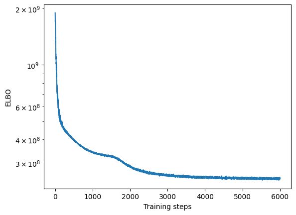
Convergence
We will first assess whether the ELBO loss of SOFA has converged by plotting it over training steps
[19]:
plt.semilogy(model.history)
plt.xlabel("Training steps")
plt.ylabel("ELBO")
[19]:
Text(0, 0.5, 'ELBO')
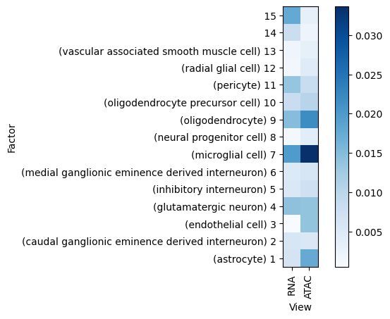
Variance explained
A good first step in a SOFA analysis is to plot how much variance is explained by each factor for each modality. This gives us an overview which factors are active across multiple modalities, capturing correlated variation across multiple measurements and which are private to a single modality, most probably capturing technical effects related to this modality.
[20]:
sofa.pl.plot_variance_explained(model)
[20]:
<Axes: xlabel='View', ylabel='Factor'>
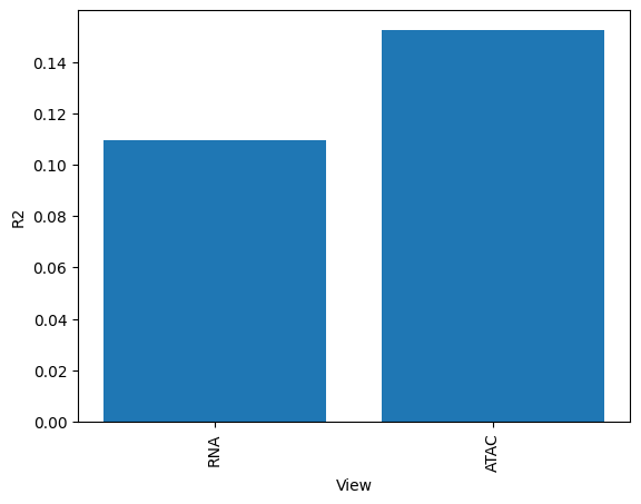
[21]:
# We can also plot how much variance of each view is explained
sofa.pl.plot_variance_explained_view(model)
[21]:
<Axes: xlabel='View', ylabel='R2'>
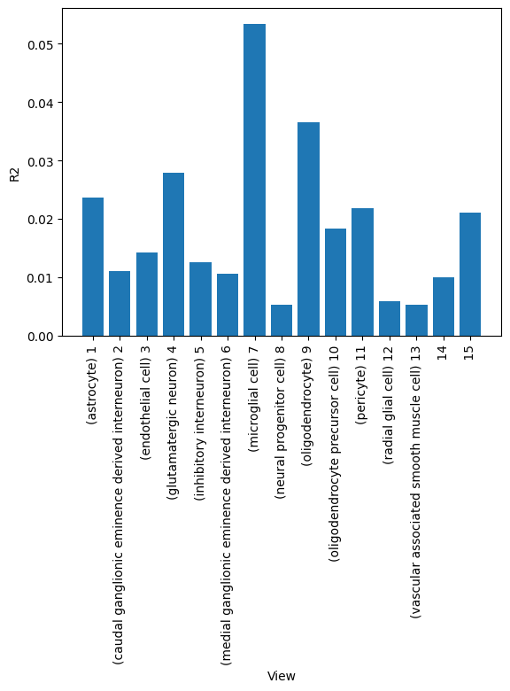
[22]:
# or how much variance is explained by each factor in total
sofa.pl.plot_variance_explained_factor(model)
[22]:
<Axes: xlabel='View', ylabel='R2'>
Check factor guidance
[23]:
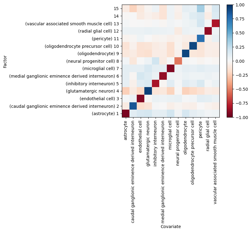
# plot correlation of factor values with cell type labels
sofa.pl.plot_factor_metadata_cor(model, celltype_df)
[23]:
<Axes: xlabel='Covariate', ylabel='Factor'>
Downstream analysis of the factor values
The factor values represent the new coordinates in lower dimensional space of our samples and have dimensions samples x factors. The factor values called Z in SOFA. We can use the factor values for all kinds of downstream analyses on the sample level. Here we will cluster the unguided factors.
We first retrieve the factor values:
[20]:
Z = sofa.tl.get_factors(model)
Z
[20]:
| Factor_1 (astrocyte) | Factor_2 (caudal ganglionic eminence derived interneuron) | Factor_3 (endothelial cell) | Factor_4 (glutamatergic neuron) | Factor_5 (inhibitory interneuron) | Factor_6 (medial ganglionic eminence derived interneuron) | Factor_7 (microglial cell) | Factor_8 (neural progenitor cell) | Factor_9 (oligodendrocyte) | Factor_10 (oligodendrocyte precursor cell) | Factor_11 (pericyte) | Factor_12 (radial glial cell) | Factor_13 (vascular associated smooth muscle cell) | Factor_14 | Factor_15 | |
|---|---|---|---|---|---|---|---|---|---|---|---|---|---|---|---|
| 4_AAACAGCCAACACTTG-1 | 0.611896 | -0.506728 | 0.283791 | 1.593037 | 0.168398 | 0.399242 | 0.422193 | 0.024536 | -0.414130 | -0.239863 | -0.121763 | 0.381870 | 0.133415 | -0.268314 | -0.236205 |
| 4_AAACAGCCACCAAAGG-1 | 0.369894 | -0.695359 | 0.196381 | 1.779255 | 0.204215 | 0.662641 | 0.385849 | -0.214301 | -0.265921 | -0.233039 | 0.073905 | 0.207890 | -0.089338 | -0.538529 | -0.470559 |
| 4_AAACAGCCATAAGTTC-1 | 0.525656 | -0.576934 | 0.151626 | 2.239841 | 0.164921 | 0.566175 | 0.381240 | -0.492999 | -0.334595 | -0.270106 | -0.003286 | 0.406507 | -0.017237 | 0.213183 | -0.319585 |
| 4_AAACATGCATAGTCAT-1 | 0.484234 | -0.433456 | 0.094686 | 1.731916 | 0.098722 | 0.500609 | 0.417679 | -0.256506 | -0.528553 | -0.414691 | -0.151233 | 0.122768 | -0.096484 | -0.026044 | -0.005257 |
| 4_AAACATGCATTGTCAG-1 | 0.473560 | -0.469949 | 0.194220 | 2.000594 | 0.305656 | 0.425527 | 0.379652 | -0.437305 | -0.143152 | -0.080377 | 0.052171 | 0.357325 | -0.041771 | -0.080069 | -0.247479 |
| ... | ... | ... | ... | ... | ... | ... | ... | ... | ... | ... | ... | ... | ... | ... | ... |
| 150666_TTTGTGAAGACAACAG-1 | 0.338253 | 0.274610 | 0.021684 | -0.642276 | 0.297069 | -0.107472 | 0.752773 | -0.331871 | 1.272615 | -0.831026 | -1.536213 | 0.170395 | 1.086244 | 0.420269 | 1.975964 |
| 150666_TTTGTGAAGGCTGTGC-1 | 0.088728 | 0.120536 | 0.196474 | -0.235622 | 0.401305 | 0.021225 | 0.439250 | -0.194579 | -1.017107 | 1.676835 | -1.030105 | 0.552844 | 0.437842 | 0.196519 | 1.003077 |
| 150666_TTTGTGAAGTAAGAAC-1 | 0.254422 | -0.270921 | 0.105018 | -0.476804 | 0.007705 | 0.118286 | 0.191205 | -0.072784 | 1.845788 | -0.173360 | -0.375505 | 0.115170 | 0.340696 | -0.138671 | 0.186792 |
| 150666_TTTGTGAAGTCTTGAA-1 | 0.707852 | -0.214515 | 0.089128 | -0.605852 | 0.340981 | 0.148991 | 0.792436 | -0.148444 | 2.024130 | -0.886393 | -1.443925 | 0.235342 | 0.654023 | 0.699232 | 1.188664 |
| 150666_TTTGTTGGTGATCAGC-1 | 0.890338 | -0.290386 | 0.247877 | -0.622976 | 0.332508 | 0.064684 | 1.110440 | -0.020911 | 2.552641 | -1.316348 | -1.953289 | 0.298762 | 1.031413 | 1.323803 | 1.993683 |
45549 rows × 15 columns
[26]:
# here we add the factors Z as obsm to the input object to be able to use scanpy for UMAP visualization
Xmdata.mod["RNA"].obsm["Z"] = Z.values
sc.pp.neighbors(Xmdata.mod["RNA"], use_rep="Z", key_added="Z_neighbors")
sc.tl.umap(Xmdata.mod["RNA"], neighbors_key="Z_neighbors", random_state=1)
[28]:
# plot the UMAP
Xmdata.mod["RNA"].obs = metadata
sc.pl.embedding(Xmdata.mod["RNA"], basis = "X_umap", color="cell_type")
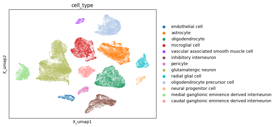
As expected the cell type separate perfectly in the UMAP visualization. This is expected as we guided the first 13 factors with the cell type labels. We can now overlay the unguided factors and check if we can identify interesting patterns:
[23]:
# add each factor as obs to the input object
Xmdata.mod["RNA"].obs = pd.concat((Xmdata.mod["RNA"].obs, Z), axis=1)
[38]:
# plot a UMAP for each factor and color by factor value
fig,axes = plt.subplots(nrows =3, ncols=5,figsize=(34,20))

axes = axes.flatten()
for i,ax in enumerate(axes):

        divnorm=mp_colors.TwoSlopeNorm(vmin=np.min(Z.iloc[:,i]), vcenter=0, vmax=np.max(Z.iloc[:,i]))
        plot = ax.scatter(Xmdata.mod["RNA"].obsm["X_umap"][:,0], Xmdata.mod["RNA"].obsm["X_umap"][:,1], c=Z.iloc[:,i], s=120000 / Xmdata.mod["RNA"].shape[0], cmap="RdBu", norm=divnorm)
        ax.set_aspect("equal")
        if model.Ymdata is not None and i < len(model.Ymdata.mod):
            covariate = list(model.Ymdata.mod.keys())[i]
            ax.set_title("Factor " +str(i+1) + " ("+ str(covariate))
        else:
            ax.set_title("Factor " +str(i+1))
        plt.colorbar(plot)
        ax.set_xlabel("UMAP 1")
        ax.set_ylabel("UMAP 2")
        ax.tick_params(
        axis='both',          # changes apply to the x-axis
        which='both',      # both major and minor ticks are affected
        bottom=False,      # ticks along the bottom edge are off
        top=False,
        left=False,# ticks along the top edge are off
        labelbottom=False,
    labelleft=False) # labels along the bottom edge are off

plt.tight_layout()
matplotlib.rcdefaults()
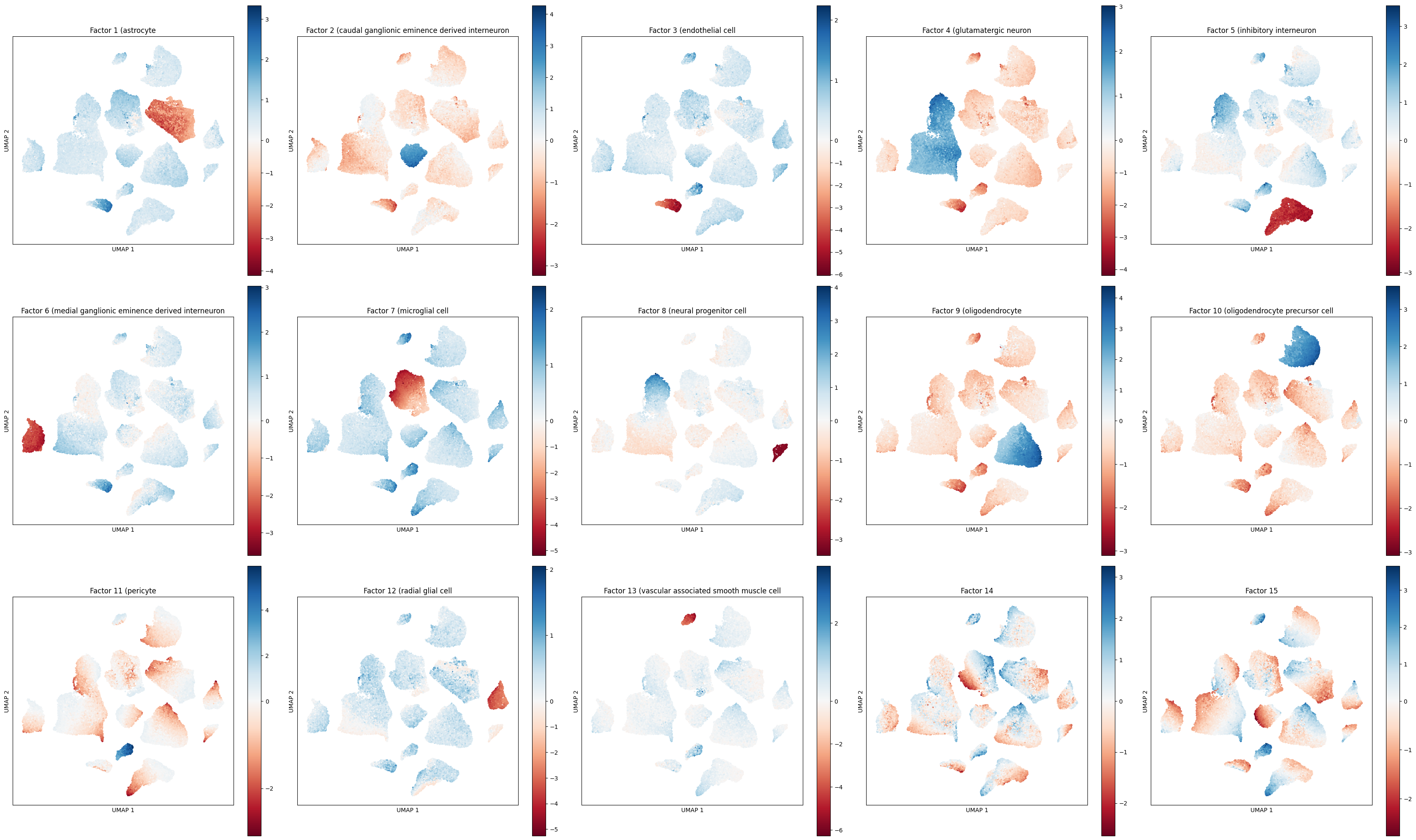
While the guided factors are active in their respective cell type clusters, the unguided factors (14 and 15) show gradients within in cell type clusters. Factor 14 shows a gradient mostly active in the microglial cell cluster.
Downstream analysis of the loadings
We will now explore what molecular features Factor 14 and Factor 15 capture.
[3]:
# specify the view of which we want to retrieve the loadings
# the loading matrix has dimensions factors x features
W_rna = sofa.tl.get_loadings(model, view="RNA")
W_rna
[3]:
| feature_name | SHOX | CSF2RA | P2RY8 | CD99 | XG | GYG2 | ARSF | MXRA5 | PRKX | STS | ... | MX2 | TMPRSS2 | TMPRSS3 | UBASH3A | TRPM2 | TSPEAR | KRTAP12-3 | ITGB2 | COL18A1 | COL6A2 |
|---|---|---|---|---|---|---|---|---|---|---|---|---|---|---|---|---|---|---|---|---|---|
| Factor_1 (astrocyte) | -0.018227 | 0.016628 | 0.008709 | -0.085218 | -0.032678 | -0.051249 | -0.128016 | -0.017553 | 0.020427 | 0.006717 | ... | -0.013714 | -0.118789 | -0.051786 | -0.068351 | -0.008388 | -0.070681 | -0.040730 | -0.034352 | -0.009784 | -0.041832 |
| Factor_2 (caudal ganglionic eminence derived interneuron) | 0.061711 | 0.025978 | 0.041309 | 0.008997 | 0.103602 | 0.066791 | 0.096115 | 0.026817 | 0.018299 | 0.073380 | ... | 0.063504 | 0.054544 | 0.064555 | 0.087258 | 0.127651 | 0.140096 | 0.034622 | 0.046414 | 0.055640 | 0.089154 |
| Factor_3 (endothelial cell) | 0.002676 | 0.046630 | -0.063564 | 0.013813 | -0.022183 | 0.019438 | 0.019055 | -0.016783 | -0.012183 | -0.014433 | ... | -0.028807 | 0.011751 | -0.020785 | -0.045028 | 0.020811 | -0.038803 | -0.009141 | 0.003219 | -0.052285 | -0.009642 |
| Factor_4 (glutamatergic neuron) | 0.044140 | -0.032026 | -0.020472 | -0.004024 | 0.047451 | 0.072089 | 0.020697 | 0.033083 | -0.000998 | 0.157253 | ... | 0.066016 | 0.010713 | 0.008618 | 0.068955 | 0.070585 | 0.160543 | 0.067635 | -0.021258 | -0.048109 | 0.078915 |
| Factor_5 (inhibitory interneuron) | 0.021449 | 0.076019 | 0.071614 | 0.111477 | 0.054973 | 0.011741 | -0.012790 | -0.002646 | -0.000420 | 0.029649 | ... | 0.103795 | 0.108892 | 0.043622 | 0.085356 | 0.144796 | 0.155512 | 0.069746 | 0.102761 | 0.190089 | 0.099793 |
| Factor_6 (medial ganglionic eminence derived interneuron) | -0.002214 | 0.011589 | 0.009022 | 0.005203 | -0.001285 | 0.022863 | 0.043369 | -0.009789 | -0.055886 | -0.051018 | ... | -0.000926 | 0.001854 | 0.013125 | -0.046666 | -0.175756 | -0.010585 | 0.021193 | 0.029928 | 0.040288 | -0.004638 |
| Factor_7 (microglial cell) | 0.033687 | -0.371200 | -0.201232 | -0.180759 | 0.048073 | 0.049734 | 0.059747 | 0.044436 | -0.062388 | 0.013768 | ... | -0.146758 | 0.037564 | 0.033068 | 0.012605 | -0.099360 | 0.029247 | 0.020464 | -0.306571 | -0.021651 | 0.055954 |
| Factor_8 (neural progenitor cell) | -0.040064 | 0.018456 | -0.022026 | 0.028713 | 0.042819 | -0.024957 | -0.036244 | -0.004213 | -0.068642 | -0.052252 | ... | 0.021161 | 0.001159 | 0.014907 | 0.055635 | 0.011421 | 0.031352 | 0.032900 | 0.015596 | -0.012561 | 0.020977 |
| Factor_9 (oligodendrocyte) | -0.045553 | -0.086439 | -0.095924 | -0.091932 | -0.071380 | -0.057834 | -0.062374 | -0.035606 | -0.074925 | -0.039691 | ... | -0.082786 | -0.074244 | -0.033555 | -0.044907 | -0.114517 | -0.094449 | -0.031309 | -0.104703 | -0.005420 | -0.073570 |
| Factor_10 (oligodendrocyte precursor cell) | 0.013328 | -0.076632 | -0.095766 | -0.061523 | 0.004489 | -0.009986 | -0.035331 | -0.014284 | -0.010431 | -0.086027 | ... | -0.005166 | 0.103091 | 0.000971 | -0.002350 | -0.054968 | -0.038637 | -0.016010 | -0.023825 | 0.012225 | -0.018629 |
| Factor_11 (pericyte) | -0.068400 | -0.117113 | -0.107469 | -0.063415 | -0.119831 | -0.101984 | -0.116682 | -0.038292 | -0.105895 | -0.142456 | ... | -0.074856 | -0.127596 | -0.068352 | -0.096209 | -0.098300 | -0.039917 | 0.005252 | -0.071315 | 0.125981 | 0.006964 |
| Factor_12 (radial glial cell) | 0.013457 | 0.035862 | 0.016619 | -0.008517 | -0.005948 | -0.048667 | -0.013628 | -0.006250 | 0.036617 | 0.091800 | ... | 0.037933 | 0.001341 | 0.018385 | 0.011399 | 0.078934 | 0.081725 | 0.034904 | 0.064347 | 0.076669 | 0.018390 |
| Factor_13 (vascular associated smooth muscle cell) | -0.020864 | -0.006278 | 0.057538 | 0.021366 | 0.016715 | -0.011897 | 0.036587 | -0.026533 | 0.022503 | 0.039456 | ... | 0.015130 | -0.010799 | 0.014685 | 0.013097 | -0.001941 | 0.011595 | 0.008483 | 0.012239 | -0.133319 | -0.082095 |
| Factor_14 | -0.030205 | -0.065338 | -0.098833 | -0.098750 | -0.020684 | 0.015680 | 0.004504 | 0.002585 | -0.049090 | 0.002668 | ... | -0.099198 | -0.061864 | -0.059691 | -0.070308 | -0.167516 | -0.050790 | -0.045526 | -0.186547 | 0.030531 | -0.045366 |
| Factor_15 | 0.102394 | 0.111089 | 0.161223 | 0.145873 | 0.143792 | 0.096924 | 0.109016 | 0.141172 | 0.169392 | 0.152441 | ... | 0.147098 | 0.099834 | 0.066984 | 0.102654 | 0.077644 | 0.146752 | 0.049644 | 0.127989 | 0.083689 | 0.177638 |
15 rows × 2000 columns
[4]:
W_atac = sofa.tl.get_loadings(model, view="ATAC")
W_atac
[4]:
| feature_name | HES5 | PRDM16 | LINC01134 | SLC2A5 | PIK3CD | TNFRSF1B | AADACL4 | SLC25A34-AS1 | PADI2 | PADI1 | ... | LINC00279 | MT-ND1 | MT-ND2 | MT-CO1 | MT-CO2 | MT-ATP6 | MT-ND3 | MT-ND4L | MT-ND4 | MT-ND5 |
|---|---|---|---|---|---|---|---|---|---|---|---|---|---|---|---|---|---|---|---|---|---|
| Factor_1 (astrocyte) | -0.208182 | -0.429047 | -0.000131 | 0.045786 | 0.080833 | 0.054359 | -0.012543 | -0.025898 | -0.091752 | 0.003296 | ... | 0.036371 | -0.049887 | -0.039553 | 0.012043 | -0.031498 | -0.078227 | -0.136771 | -0.020041 | -0.042751 | -0.024138 |
| Factor_2 (caudal ganglionic eminence derived interneuron) | -0.036767 | -0.069018 | 0.001598 | -0.011377 | -0.025387 | -0.038779 | 0.004101 | 0.004330 | -0.035379 | 0.003445 | ... | 0.001888 | 0.138144 | 0.123199 | 0.152745 | 0.134151 | 0.095955 | 0.093427 | 0.094417 | 0.135157 | 0.092551 |
| Factor_3 (endothelial cell) | 0.026845 | 0.086176 | -0.006730 | 0.032492 | 0.092398 | -0.062162 | 0.009899 | 0.019996 | 0.012182 | 0.006935 | ... | 0.010711 | 0.007029 | -0.003770 | 0.000740 | 0.000596 | -0.013372 | -0.011830 | 0.009384 | -0.013850 | -0.012648 |
| Factor_4 (glutamatergic neuron) | -0.119810 | -0.110515 | -0.008428 | -0.065243 | -0.076141 | -0.082045 | 0.001842 | -0.012405 | -0.123653 | -0.004981 | ... | -0.027927 | -0.064613 | -0.099515 | -0.053974 | -0.108447 | -0.121445 | -0.160079 | -0.058071 | -0.102936 | -0.070332 |
| Factor_5 (inhibitory interneuron) | 0.074077 | 0.080980 | -0.000610 | 0.054926 | 0.059176 | 0.070569 | -0.001754 | -0.002609 | 0.111904 | 0.008717 | ... | 0.032175 | 0.144616 | 0.140038 | 0.144284 | 0.186204 | 0.150951 | 0.152748 | 0.052082 | 0.145854 | 0.084795 |
| Factor_6 (medial ganglionic eminence derived interneuron) | 0.061534 | 0.110697 | -0.012850 | 0.014597 | -0.108322 | 0.006335 | -0.001688 | 0.008390 | 0.036388 | -0.003137 | ... | 0.001910 | -0.249092 | -0.228440 | -0.332192 | -0.354922 | -0.283303 | -0.202077 | -0.081255 | -0.252142 | -0.182548 |
| Factor_7 (microglial cell) | 0.073273 | 0.076353 | -0.015753 | -0.372691 | -0.235887 | -0.319122 | -0.010101 | -0.001108 | -0.065391 | -0.022516 | ... | 0.011044 | 0.019545 | 0.015750 | 0.001131 | 0.000565 | -0.025114 | -0.020271 | 0.019034 | 0.008098 | 0.033560 |
| Factor_8 (neural progenitor cell) | 0.094023 | -0.073044 | -0.020015 | -0.010783 | 0.006819 | -0.035352 | -0.022101 | 0.004570 | 0.003941 | 0.013296 | ... | 0.004650 | 0.018530 | 0.006067 | 0.097694 | 0.021061 | -0.002756 | -0.011136 | -0.008039 | 0.041842 | 0.008941 |
| Factor_9 (oligodendrocyte) | -0.096187 | -0.090426 | 0.002811 | -0.057448 | -0.100601 | -0.064315 | 0.001830 | 0.006622 | 0.256400 | 0.001876 | ... | 0.140956 | -0.023779 | 0.035511 | 0.045417 | 0.096452 | 0.008418 | 0.016682 | -0.010833 | 0.055347 | -0.018010 |
| Factor_10 (oligodendrocyte precursor cell) | 0.109106 | -0.139850 | -0.001256 | -0.085660 | -0.103560 | -0.073114 | -0.011707 | -0.001273 | -0.034249 | 0.001216 | ... | -0.023487 | -0.091286 | -0.058322 | -0.080787 | -0.033584 | -0.034352 | -0.039314 | -0.031082 | -0.040277 | -0.050600 |
| Factor_11 (pericyte) | -0.096806 | -0.082905 | -0.013746 | -0.031378 | 0.182597 | 0.024180 | 0.004992 | 0.009840 | -0.045573 | 0.001019 | ... | -0.022335 | 0.069674 | 0.102980 | 0.051257 | 0.088180 | 0.073444 | 0.077907 | 0.039346 | 0.044237 | 0.039888 |
| Factor_12 (radial glial cell) | -0.305815 | -0.370938 | 0.014988 | 0.027542 | 0.026361 | 0.024751 | -0.001839 | 0.037604 | 0.079338 | 0.000370 | ... | 0.007548 | 0.139923 | 0.137401 | 0.122713 | 0.170129 | 0.160537 | 0.122313 | 0.048193 | 0.146312 | 0.089201 |
| Factor_13 (vascular associated smooth muscle cell) | 0.097635 | 0.021009 | -0.025192 | 0.014730 | 0.082244 | 0.057195 | -0.006985 | -0.018558 | 0.041190 | -0.010776 | ... | 0.011489 | 0.117726 | 0.129374 | 0.112941 | 0.148383 | 0.155056 | 0.177456 | 0.069603 | 0.138858 | 0.053408 |
| Factor_14 | 0.064157 | -0.044716 | -0.024030 | 0.007258 | 0.054465 | -0.057635 | 0.013054 | -0.013529 | 0.020315 | 0.006386 | ... | 0.040675 | -0.076650 | -0.030133 | -0.004744 | -0.037376 | -0.099526 | -0.079796 | 0.008935 | -0.054390 | -0.010699 |
| Factor_15 | 0.004490 | -0.062551 | 0.004475 | 0.026869 | 0.085769 | 0.083807 | 0.021577 | -0.018813 | -0.007668 | -0.005300 | ... | -0.029235 | 0.010413 | 0.031491 | 0.010445 | 0.000602 | 0.039254 | 0.070796 | -0.004739 | 0.025249 | -0.005580 |
15 rows × 2000 columns
To plot the top loadings use:
[31]:
# plot the top negative RNA loadings of Factor 7 (microglial cells)
sofa.pl.plot_top_loadings(model, view="RNA", factor = 7, top_n=20, sign="-")
[31]:
<Axes: xlabel='Loadings', ylabel='Features'>
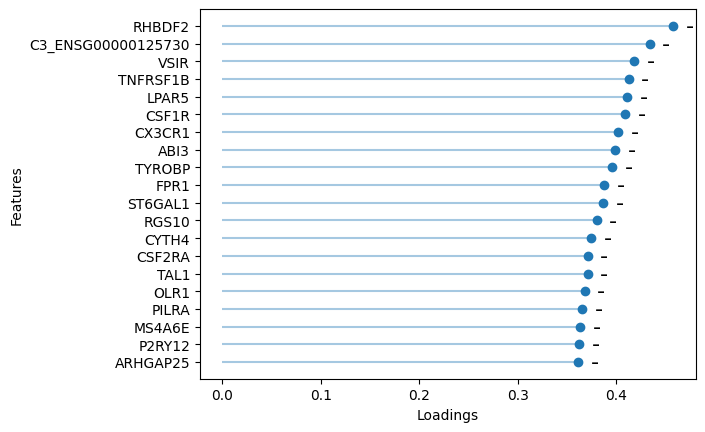
Among the top loadings of Factor 7 (guided by microglial cell label) are markers for microglial cells (CSF1R, CX3CR1, TYROBP).
Gene set overrepresentation analysis
We can use gene set overrepresentation analysis on the top loadings of a given factor. Factors typically represent axes of variation having a positive and a negative end. We will therefore both investigate the positive or negative loadings. This gives us an overview of which gene sets are enriched in this factor and what biological processes it probably captured.
Factor 14
[20]:
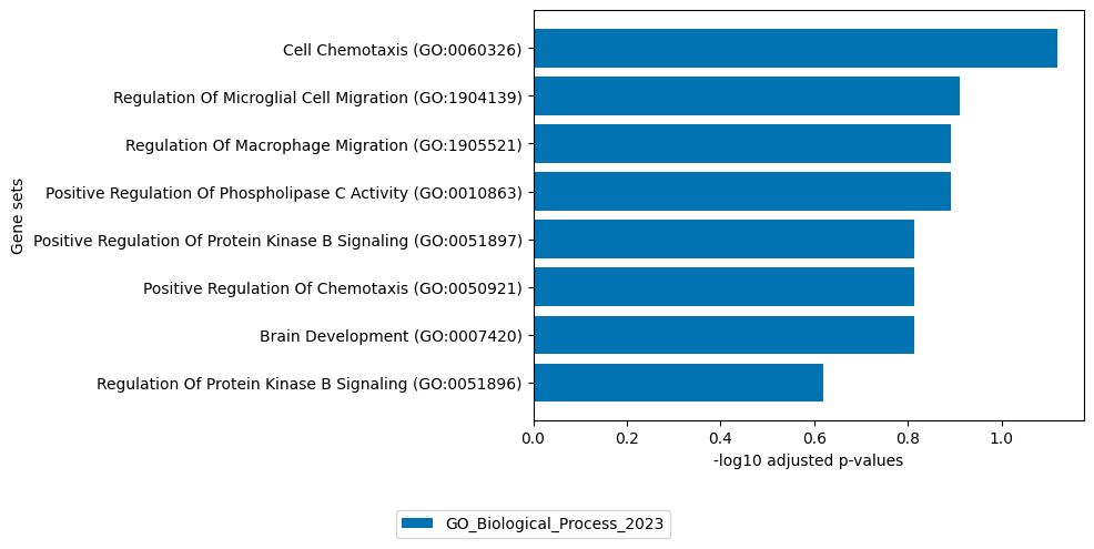
# get top 100 positive loadings of ATAC view
loadings = sofa.tl.get_top_loadings(model,factor=14, view="ATAC", sign="+", top_n=100)


sofa.pl.plot_enrichment(loadings,
                        background=Xmdata.mod["ATAC"].var, # all genes considered in the analysis, used as background
                        db=[ "GO_Biological_Process_2023"],  # a list of databases for overrepresentation analysis,
                        top_n=[8]) # the number of genesets for each database to plot
# sofa.pl.plot_enrichment uses the enrichr API, please refer to https://maayanlab.cloud/Enrichr/#libraries for a full list of available databases
[20]:
<Axes: xlabel='-log10 adjusted p-values', ylabel='Gene sets'>
[21]:
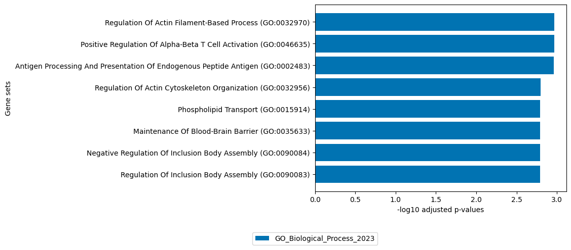
# get top 100 negative loadings of ATAC view
loadings = sofa.tl.get_top_loadings(model,factor=14, view="ATAC", sign="-", top_n=100)


sofa.pl.plot_enrichment(loadings,
                        background=Xmdata.mod["ATAC"].var, # all genes considered in the analysis, used as background
                        db=["GO_Biological_Process_2023"],  # a list of databases for overrepresentation analysis,
                        top_n=[8]) # the number of genesets for each database to plot
# sofa.pl.plot_enrichment uses the enrichr API, please refer to https://maayanlab.cloud/Enrichr/#libraries for a full list of available databases
[21]:
<Axes: xlabel='-log10 adjusted p-values', ylabel='Gene sets'>
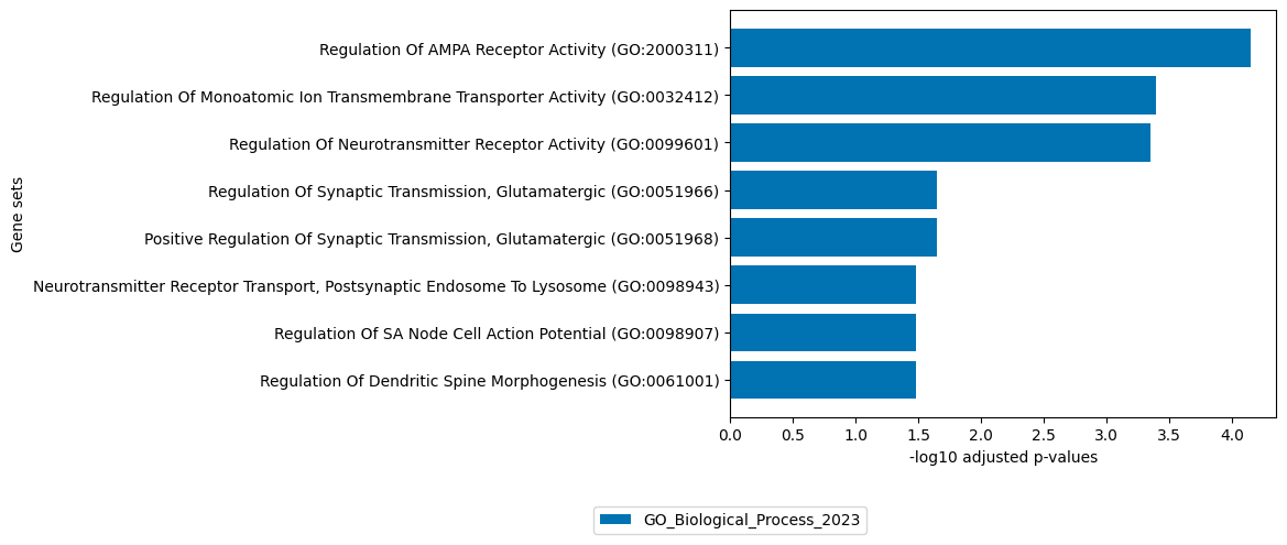
Factor 15
[23]:
# get top 100 positive loadings of RNA view
loadings = sofa.tl.get_top_loadings(model,factor=15, view="RNA", sign="+", top_n=100)


sofa.pl.plot_enrichment(loadings,
                        background=Xmdata.mod["RNA"].var, # all genes considered in the analysis, used as background
                        db=["GO_Biological_Process_2023"],  # a list of databases for overrepresentation analysis,
                        top_n=[8]) # the number of genesets for each database to plot
# sofa.pl.plot_enrichment uses the enrichr API, please refer to https://maayanlab.cloud/Enrichr/#libraries for a full list of available databases
[23]:
<Axes: xlabel='-log10 adjusted p-values', ylabel='Gene sets'>
[24]:
# get top 100 negative loadings of RNA view
loadings = sofa.tl.get_top_loadings(model,factor=15, view="RNA", sign="-", top_n=100)


sofa.pl.plot_enrichment(loadings,
                        background=Xmdata.mod["RNA"].var, # all genes considered in the analysis, used as background
                        db=["GO_Biological_Process_2023"],  # a list of databases for overrepresentation analysis,
                        top_n=[8]) # the number of genesets for each database to plot
# sofa.pl.plot_enrichment uses the enrichr API, please refer to https://maayanlab.cloud/Enrichr/#libraries for a full list of available databases
[24]:
<Axes: xlabel='-log10 adjusted p-values', ylabel='Gene sets'>
